Why Learn Machine Learning?
Machine Learning (ML) is currently one of the most talked about topics in the field of technology and will remain so for the coming years. The reasons for this are:
- A high amount of data is being produced today by us in the form of text, images, videos, geolocations, and many more.
- Increase in computation power, thus leading to higher speed and lower cost of analysis of the data.
- The development of better algorithms leads to better analysis, better prediction power, and higher accuracy.
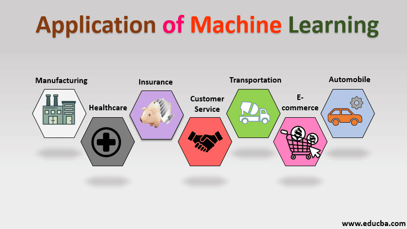
Today Machine Learning is being used everywhere, from mundane to high-end applications.
A few examples of mundane applications of Machine Learning are:
- Google search and page ranking
- Recommendation engines for youtube videos, amazon shopping, etc.
- Face detection in image tagging
- Language translation (using Google Translate)
A few examples of high-end applications of Machine Learning are:
- Cancer detection from X-ray images
- Self-driving cars for automatic navigation
- Aircraft Control for altitude adjustment
- Computer vision in manufacturing, such as detecting defective samples
- Computer vision in security systems for threat detection
Machine Learning is a continuously developing field that will keep covering more and more areas of applications in the coming years and will also keep improving its performance in all of those areas, thus driving technological progress and business growth.
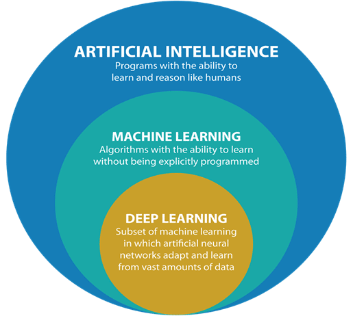
What is Machine Learning?
- Machine Learning is a sub-field of Artificial intelligence. Machine Learning itself can have other sub-fields such as Deep Learning which is a class of machine learning algorithms that are inspired by the human brain.

- Although AI and hence machine learning is a field within computer science, it differs from traditional computational approaches:
- In traditional computing, algorithms are step-wise instructions that are programmed explicitly by us and used by computers to solve a problem.
- On the other hand, Machine Learning algorithms learn from the data provided to them, using a statistical analysis/modeling approach and make their own set of rules. The ML algorithm can then make decisions based on this set of rules that it learned from the data.
Introduction to Image Classifier
The Image Classifier of the PictoBlox Machine Learning Environment is used for classifying images into different classes based on their characteristics.
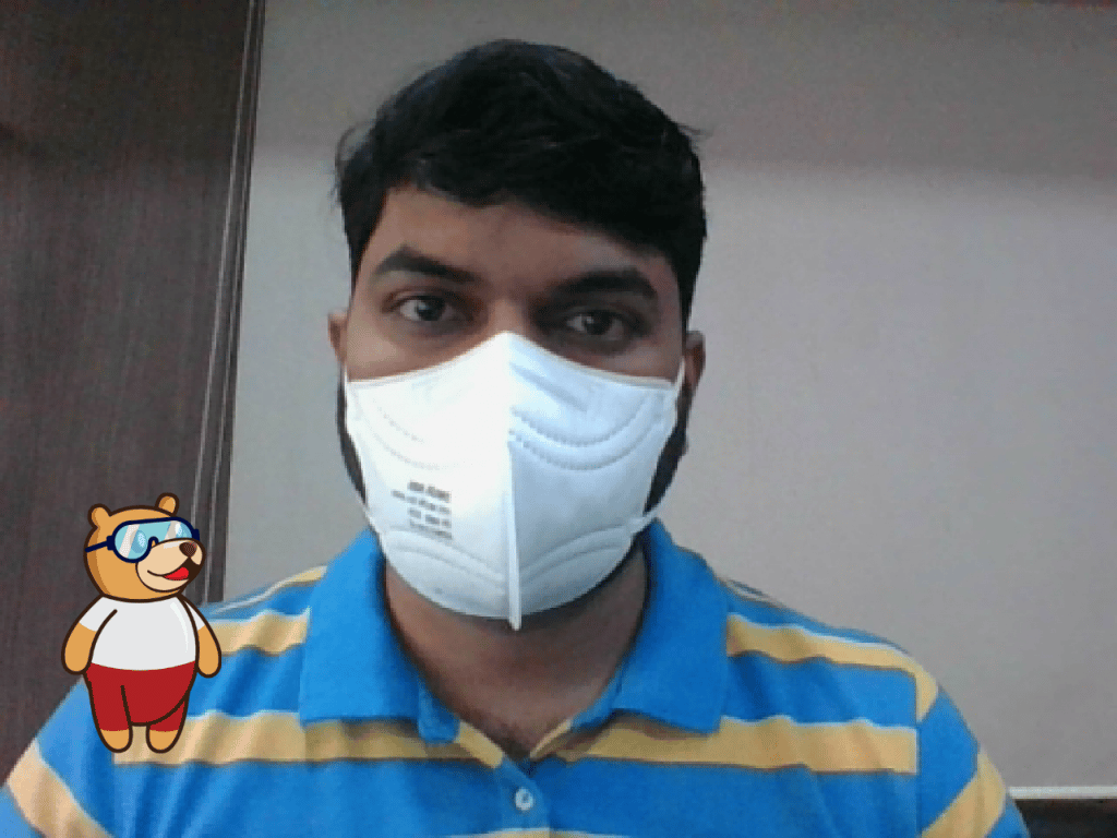
For example, let’s say you want to construct a model to judge if a person is wearing a mask correctly or not, or if the person’s wearing one at all. You’ll have to classify your image into three classes:
- Wearing mask

- Not wearing mask
- Wearing mask incorrectly


This is the case of image classification where you want the machine to label the images into one of the classes.
In this tutorial, we’ll learn how to construct the ML model using the PictoBlox Image Classifier.
Following are the steps involved in the procedure:
- Setting up the environment
- Gathering the data (Data collection)
- Training the model
- Testing the model
- Exporting the model to PictoBlox
- Creating a script in PictoBlox
Setting up the Environment
First, we need to set the ML environment for image classification.

Follow the steps below:
- Open PictoBlox and create a new file.

- Select the coding environment as Python Coding.

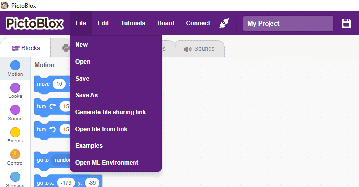
- To access the ML Environment, select the “Open ML Environment” option under the “File” tab.

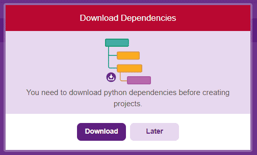
- You have to download the Python Dependencies when you execute it the first time. The following window will open. Click on the Download button and wait for the dependencies to download.

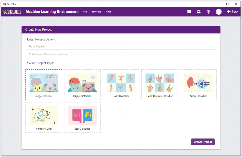
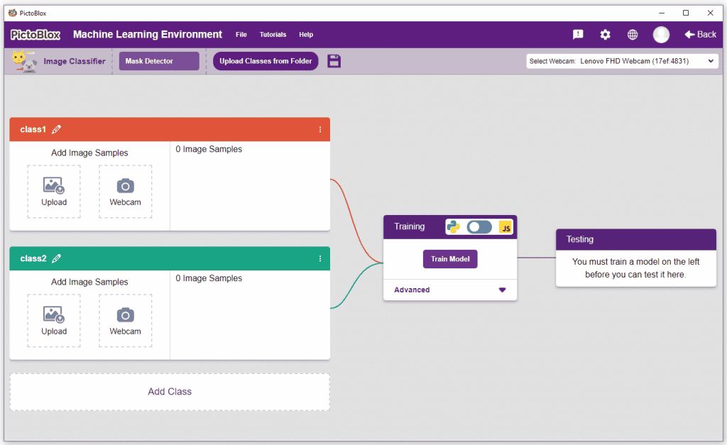
- You’ll be greeted with the following screen.
 Click on “Create New Project“.
 - A window will open. Type in a project name of your choice and select the “Image Classifier” extension. Click the “Create Project” button to open the Image Classifier window.

- You shall see the Image Classifier Workflow with two classes already made for you. Your environment is all set. Now it’s time to upload the data.


Collecting and Uploading the Data
Each class is a specific category. The Machine Learning model classifies the images into such two or more classes. Similar images are put in the same class.
There are 2 things that you need to provide in each class:
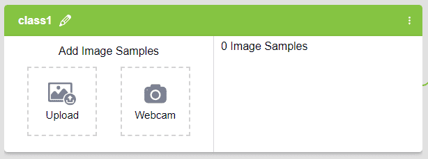
- Class Name: Write a name at the place “class1” is written, by clicking on the pencil icon.
- Image Data: This data can either be taken from the webcam (Webcam button) or by uploading (Upload button) from local storage or from google drive.
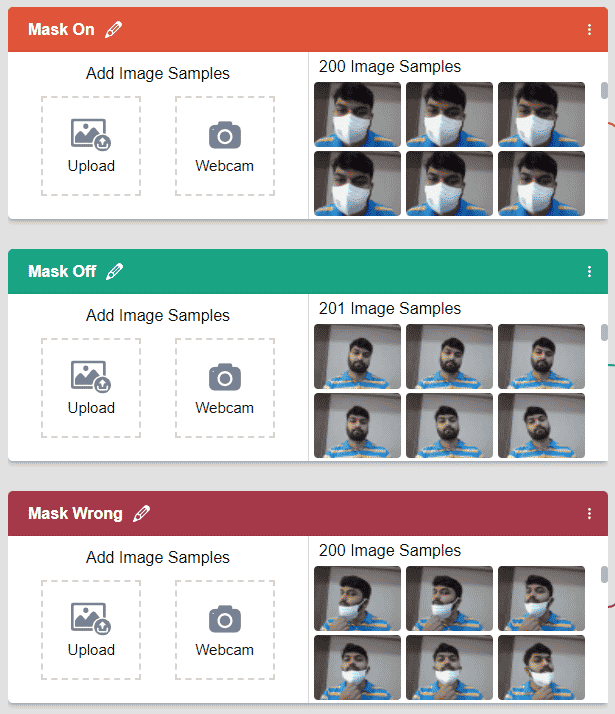
For this project, we’ll be needing three classes:
- Wearing mask – Mask On
- Not wearing a mask – Mask Off
- Wearing mask incorrectly – Mask Wrong
Follow below given steps, to upload the data for the three classes:
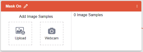
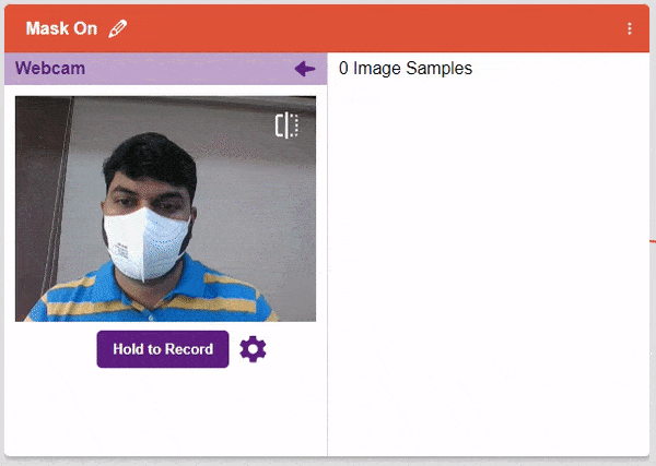
- Rename the first class: Mask On.

- Click the Webcam button.
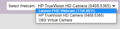
If you want to change your camera feed, you can do it from the webcam selector in the top right corner.

- Next, click on the “Hold to Record” button to capture the with mask images. Take 200 photos with different head orientations.
 If you want to delete any image, then hover over the image and click on the delete button.
 Once uploaded, you will be able to see the images in the class.
 - Rename Class 2 as Mask Off and take the samples from the webcam.

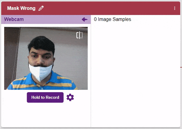
- Click the “Add Class” button, and you shall see a new class in your Environment. Rename the class name to Mask Wrong.

 Note: You must add at least 20 samples to each of your classes for your model to train. More samples will lead to better results.
 - As you can see, now each class has some data to derive patterns from. In order to extract and use these patterns, we must train our model.
 If you want to delete any image, then hover over the image and click on the delete button.
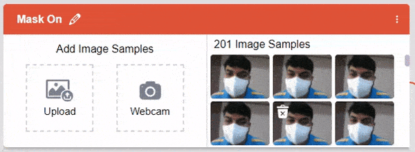 Once uploaded, you will be able to see the images in the class.
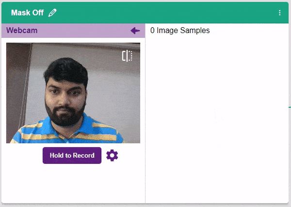
Training the Model
Now that we have gathered the data, it’s time to teach our model how to classify new, unseen data into these three classes. In order to do this, we have to train the model. By training the model, we extract meaningful information from the images, and that in turn updates the weights. Once these weights are saved, we can use our model to make predictions on data previously unseen.
However, before training the model, there are a few hyperparameters that you should be aware of. Click on the “Advanced” tab to view them.
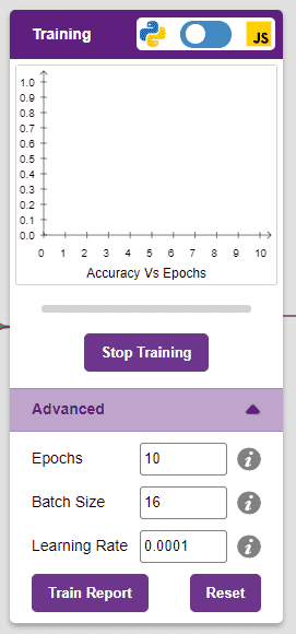

There are three hyperparameters you can play along with here:
- Epochs– The total number of times your data will be fed through the training model. Therefore, in 10 epochs, the dataset will be fed through the training model 10 times. Increasing the number of epochs can often lead to better performance.
- Batch Size– The size of the set of samples that will be used in one step. For example, if you have 160 data samples in your dataset, and you have a batch size of 16, each epoch will be completed in 160/16=10 steps. You’ll rarely need to alter this hyperparameter.
- Learning Rate– It dictates the speed at which your model updates the weights after iterating through a step. Even small changes in this parameter can have a huge impact on the model performance. The usual range lies between 0.001 and 0.0001.
Let’s train the model with the standard hyperparameters and see how it performs. You can train the model only in Python (not in JS), since you are working in Python Coding Environment.
Click on the “Train Model” button to commence training. We need not change any hyperparameter for this model.

The model shows great results! Remember, the higher the reading in the accuracy graph, better the model. The x-axisof the graph shows the epochs, and the y-axis represents the corresponding accuracy. The range of the accuracy is 0 to 1.
Testing the Model
Now that the model is trained, let us see if it delivers the expected results. We can test the model by either using the device’s camera or by uploading an image from the device’s storage. Let’s use our webcam to start with.
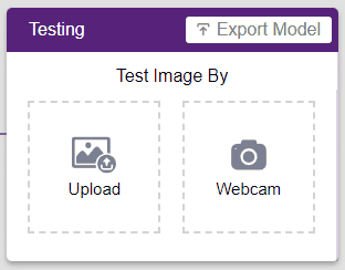
Click on the “Webcam” option in the testing box and the model will start predicting based on the image in the window.
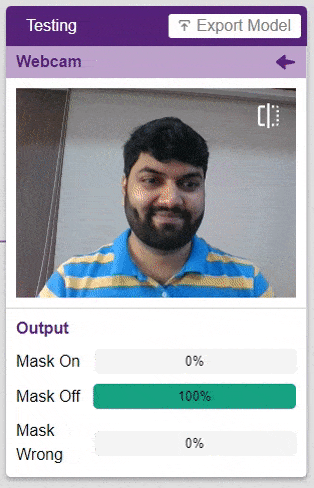
Great! The model is able to make predictions in real-time. Now close the window by clicking on the cross on the top right of the testing box.
Now we can export our model and make a project in the Python coding environment.
Exporting the Model to the Python Environment

Click on the “Export Model” button on the top right of the Testing box, and PictoBlox will load your model into the Python Environment.
Observe that a python testing code will automatically appear in the scripting area, ready for you to test.
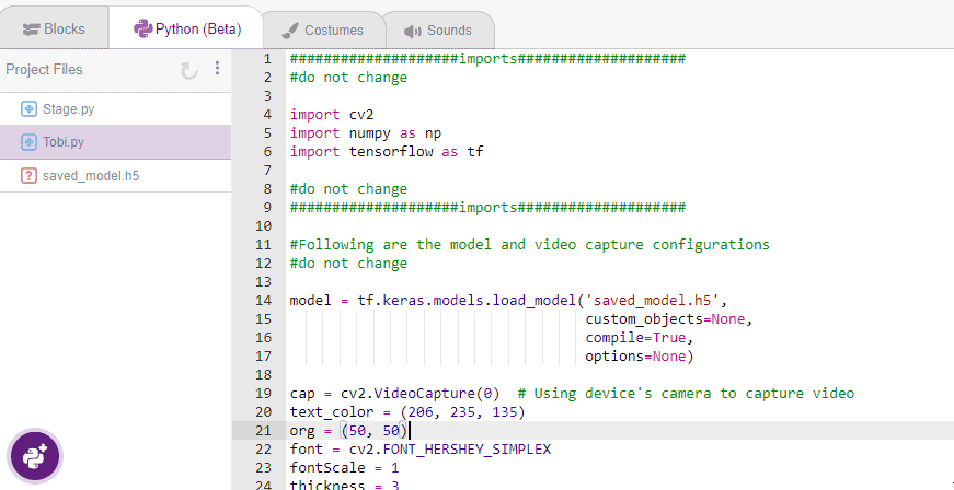
Click on Beautify Button to make the code error-free of any indentation errors. It’s the left icon from the A+ icon (Magic Wand).
Following is the code which is created by PictoBlox.
####################imports####################
#do not change

import cv2
import numpy as np
import tensorflow as tf

#do not change
####################imports####################

# Following are the model and video capture configurations
# do not change

model = tf.keras.models.load_model('saved_model.h5',
                                   custom_objects=None,
                                   compile=True,
                                   options=None)

cap = cv2.VideoCapture(0)  # Using device's camera to capture video
text_color = (206, 235, 135)
org = (50, 50)
font = cv2.FONT_HERSHEY_SIMPLEX
fontScale = 1
thickness = 3

class_list = ['Mask Off', 'Mask On', 'Mask Wrong']  # List of all the classes

#do not change
###############################################

#This is the while loop block, computations happen here

while True:
  ret, image_np = cap.read()  # Reading the captured images
  image_np = cv2.flip(image_np, 1)
  image_resized = cv2.resize(image_np, (224, 224))
  img_array = tf.expand_dims(image_resized,
                             0)  # Expanding the image array dimensions
  predict = model.predict(img_array)  # Making an initial model prediction
  predict_index = np.argmax(predict[0],
                            axis=0)  # Generating index out of the prediction
  predicted_class = class_list[
      predict_index]  # Tallying the index with class list

  image_np = cv2.putText(
      image_np, "Image Classification Output: " + str(predicted_class), org,
      font, fontScale, text_color, thickness, cv2.LINE_AA)

  print(predict)
  cv2.imshow("Image Classification Window",
             image_np)  # Displaying the classification window

  ###############################################
  #Add your code here

  #Add your code here
  ###############################################

  if cv2.waitKey(25) & 0xFF == ord(
      'q'):  # Press 'q' to close the classification window
    break

cap.release()  # Stops taking video input
cv2.destroyAllWindows()  #Closes input window
The code uses three libraries:
- OpenCV – For image capture and image processing
- Numpy – For array manipulation
- Tensorflow – For machine learning
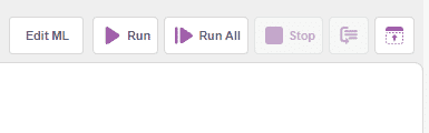
Click on the Run button to run and test the code.